
Average over several test sets
Source:vignettes/articles/howto-multiple-test-sets.Rmd
howto-multiple-test-sets.RmdOne model tested on several datasets gives several curves.
precrec averages them and draws a confidence band around
the average.
library(precrec)
library(ggplot2)

# 10 test sets for one model
samps <- create_sim_samples(10, 100, 100, "good_er")

mdat <- mmdata(samps[["scores"]], samps[["labels"]], dsids = samps[["dsids"]])
dsids is what marks these as several test sets rather
than several models.
The average curve
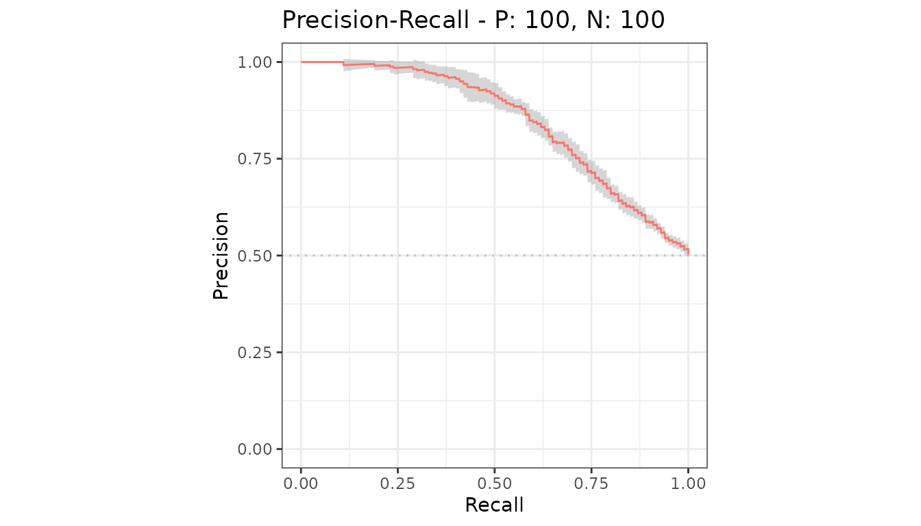
The shaded band is the point-wise 95% confidence interval of the average. It appears on its own as soon as a model has more than one test set.
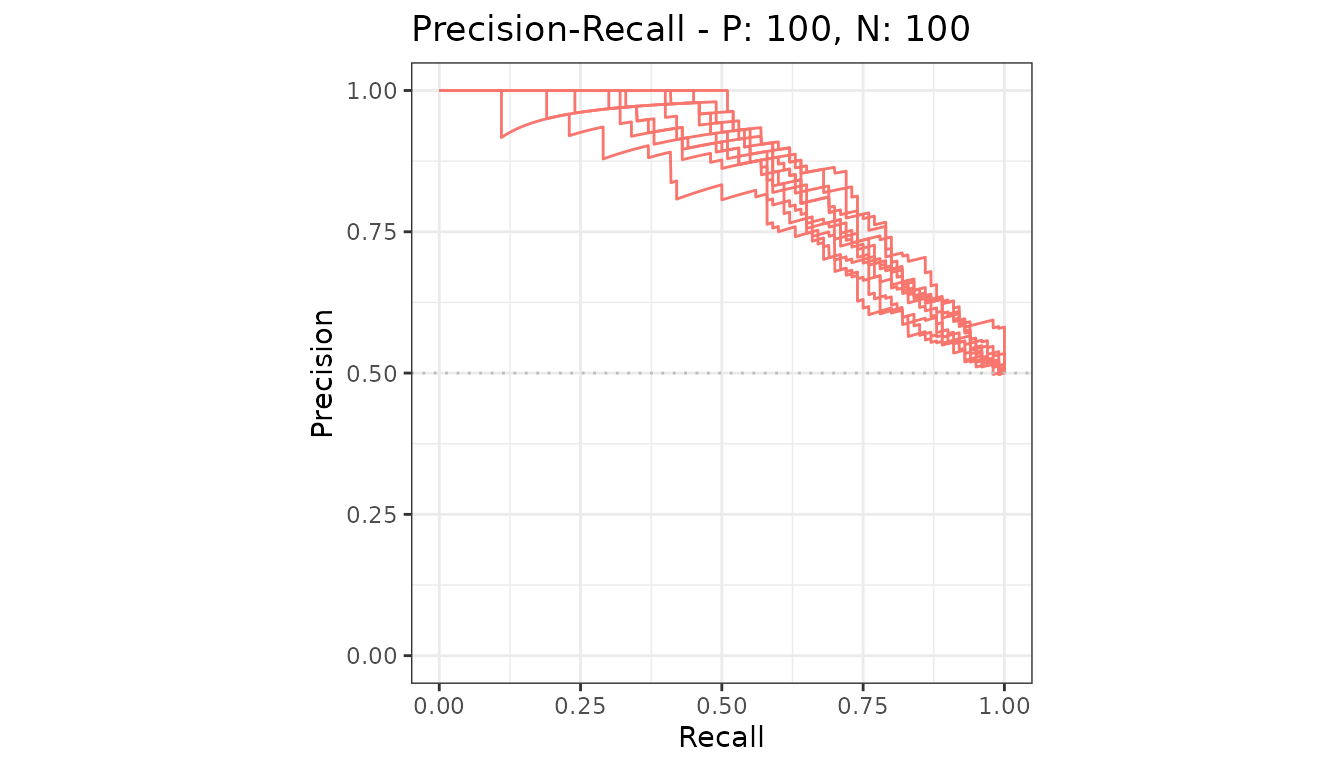
Averaged areas
auc() reports the mean area over the test sets.
| modnames | dsids | curvetypes | aucs | baselines |
|---|---|---|---|---|
| m1 | 1 | ROC | 0.8180000 | 0.5 |
| m1 | 1 | PRC | 0.8574152 | 0.5 |
| m1 | 2 | ROC | 0.7865000 | 0.5 |
| m1 | 2 | PRC | 0.8404735 | 0.5 |
| m1 | 3 | ROC | 0.8313000 | 0.5 |
| m1 | 3 | PRC | 0.8628264 | 0.5 |
| m1 | 4 | ROC | 0.8244000 | 0.5 |
| m1 | 4 | PRC | 0.8578336 | 0.5 |
| m1 | 5 | ROC | 0.8204000 | 0.5 |
| m1 | 5 | PRC | 0.8519919 | 0.5 |
| m1 | 6 | ROC | 0.8285000 | 0.5 |
| m1 | 6 | PRC | 0.8577692 | 0.5 |
| m1 | 7 | ROC | 0.7925000 | 0.5 |
| m1 | 7 | PRC | 0.8071713 | 0.5 |
| m1 | 8 | ROC | 0.7832000 | 0.5 |
| m1 | 8 | PRC | 0.8267456 | 0.5 |
| m1 | 9 | ROC | 0.8343000 | 0.5 |
| m1 | 9 | PRC | 0.8609178 | 0.5 |
| m1 | 10 | ROC | 0.7943000 | 0.5 |
| m1 | 10 | PRC | 0.8497775 | 0.5 |
auc_ci() puts a confidence interval on it.
| modnames | curvetypes | mean | baselines | error | lower_bound | upper_bound | n |
|---|---|---|---|---|---|---|---|
| m1 | ROC | 0.8113400 | 0.5 | 0.0123463 | 0.7989937 | 0.8236863 | 10 |
| m1 | PRC | 0.8472922 | 0.5 | 0.0110427 | 0.8362495 | 0.8583350 | 10 |
Both at once
Several models and several test sets is the same call with both identifiers set. Each model gets one average curve.
samps2 <- create_sim_samples(10, 100, 100, c("poor_er", "good_er"))

mdat2 <- mmdata(samps2[["scores"]], samps2[["labels"]],
  modnames = samps2[["modnames"]], dsids = samps2[["dsids"]]
)

autoplot(evalmod(mdat2), "PRC")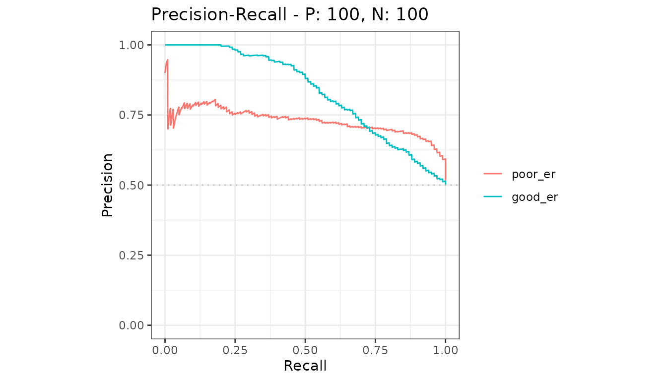
Next
- Confidence bands - how the band is built and how to change it
- Evaluate cross-validation folds