Confusion-matrix rates

Everything here is a ratio of two cells of the 2x2 table, evaluated at every cutoff.

	Predicted positive	Predicted negative
Actually positive	TP	FN
Actually negative	FP	TN

library(precrec)
library(ggplot2)

points <- evalmod(
  scores = P10N10$scores, labels = P10N10$labels,
  mode = "basic"
)

Overall

Metric	Formula	Range
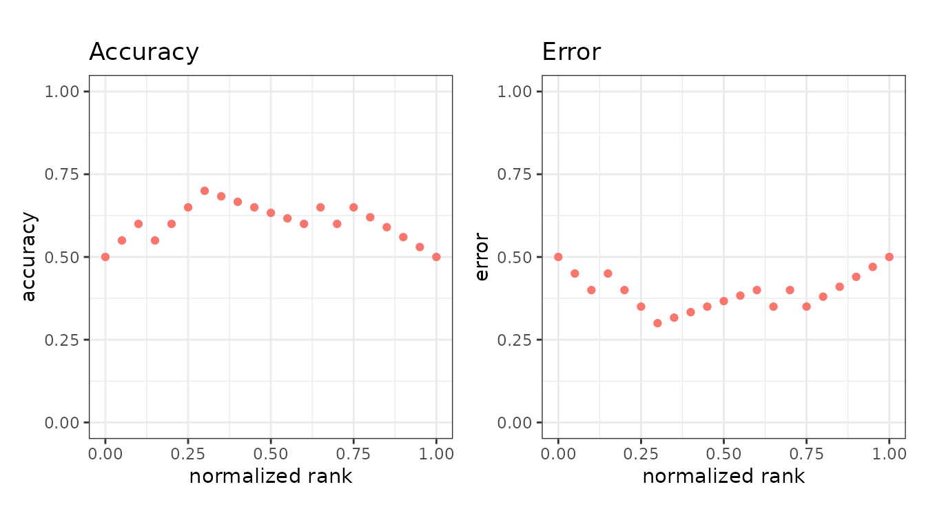
`accuracy`	(TP + TN) / all	0 to 1
`error`	(FP + FN) / all	0 to 1

Accuracy is the metric to distrust first. On data with 1% positives, calling everything negative scores 0.99.

autoplot(points, c("accuracy", "error"))

Rates over the actual classes

These divide by a row, so they do not move when the class balance changes.

Metric	Formula	Also known as
`sensitivity`	TP / (TP + FN)	recall, TPR, hit rate
`specificity`	TN / (TN + FP)	TNR, selectivity
`fpr`	FP / (FP + TN)	fall-out, 1 - specificity
`fnr`	FN / (TP + FN)	miss rate, 1 - sensitivity

The ROC curve is sensitivity against fpr, which is why it is blind to class balance - both axes are row-wise rates.

Rates over the predicted classes

These divide by a column, so they do move with the class balance - what makes them informative on imbalanced data, and impossible to transfer between datasets.

Metric	Formula	Also known as
`precision`	TP / (TP + FP)	PPV
`npv`	TN / (TN + FN)	negative predictive value
`false_discovery_rate`	FP / (TP + FP)	1 - precision
`false_omission_rate`	FN / (TN + FN)	1 - NPV

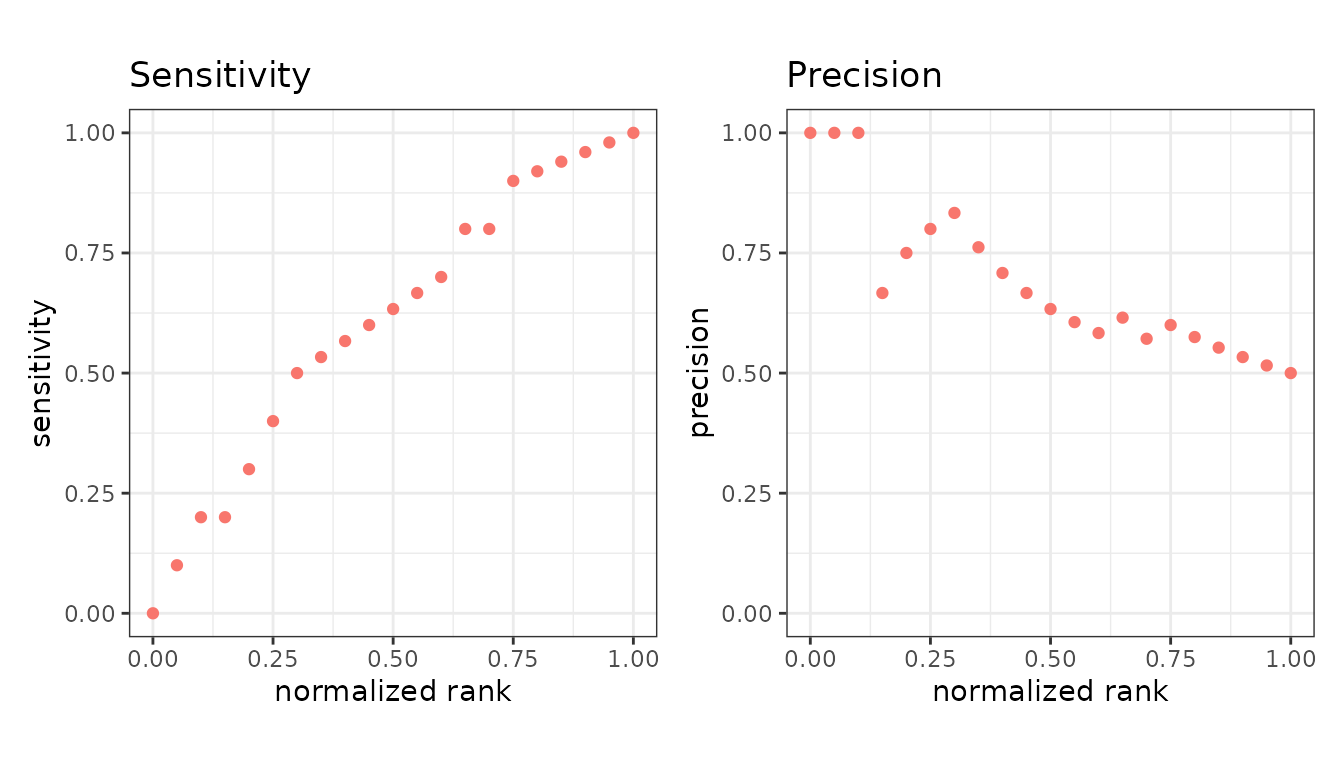
autoplot(points, c("sensitivity", "precision"))

The precision-recall curve is precision against sensitivity - one column-wise rate against one row-wise rate. See imbalanced data.

How much gets flagged

Metric	Formula	Also known as
`predicted_positive_rate`	(TP + FP) / all	rate of positive predictions
`predicted_negative_rate`	(TN + FN) / all	rate of negative predictions

Useful when review cost is the constraint: they say how much work a cutoff creates, regardless of whether the work is well spent.

Leaving out the true negatives

Metric	Formula	Also known as
`jaccard`	TP / (TP + FP + FN)	critical success index, threat score

The 2x2 table with one corner deleted. The true negatives do not count, the same omission precision and sensitivity make, which is why the three move together on imbalanced data while accuracy does not.

Pad the dataset with 200 negatives that score below everything real, and nothing about its handling of the positives has changed:

best <- function(s, l, m) {
  df <- as.data.frame(evalmod(
    scores = s, labels = l, mode = "basic",
    metrics = m
  ))
  max(df$y[df$type == m], na.rm = TRUE)
}

pad_s <- c(P10N10$scores, rep(0, 200))
pad_l <- c(P10N10$labels, rep(-1, 200))

c(
  jaccard = best(pad_s, pad_l, "jaccard"),
  accuracy = best(pad_s, pad_l, "accuracy")
)
#>   jaccard  accuracy 
#> 0.5625000 0.9727273

jaccard holds at 0.5625; accuracy climbs from 0.70, because most of what it now counts is the padding. Forecast verification calls this the critical success index for the same reason: a rare event has so many true negatives that any metric counting them reports mostly the rarity.

Undefined ends