
Six measures that answer questions the confusion-matrix rates do not:
how much better than random is this cutoff, how much does it cost, how
much does it tell us. All six are opt-in through
metrics =.
library(precrec)
library(ggplot2)

samps <- create_sim_samples(1, 100, 100, "good_er")
Lift and odds
| Measure | Formula | Range |
|---|---|---|
lift |
sensitivity / rate of positive predictions | 0 upward |
odds |
(TP x TN) / (FN x FP) | 0 upward |
Lift is how many times better than random selection the cutoff is: a lift of 3 means the flagged group holds three times the share of positives the whole dataset does. It is the standard measure in marketing and screening, where the question is what to do with a limited review budget.
The odds ratio is the odds of being positive among the flagged against the odds among the rest.
points <- evalmod(
  scores = samps$scores, labels = samps$labels,
  mode = "basic", metrics = c("lift", "odds")
)

autoplot(points, "lift")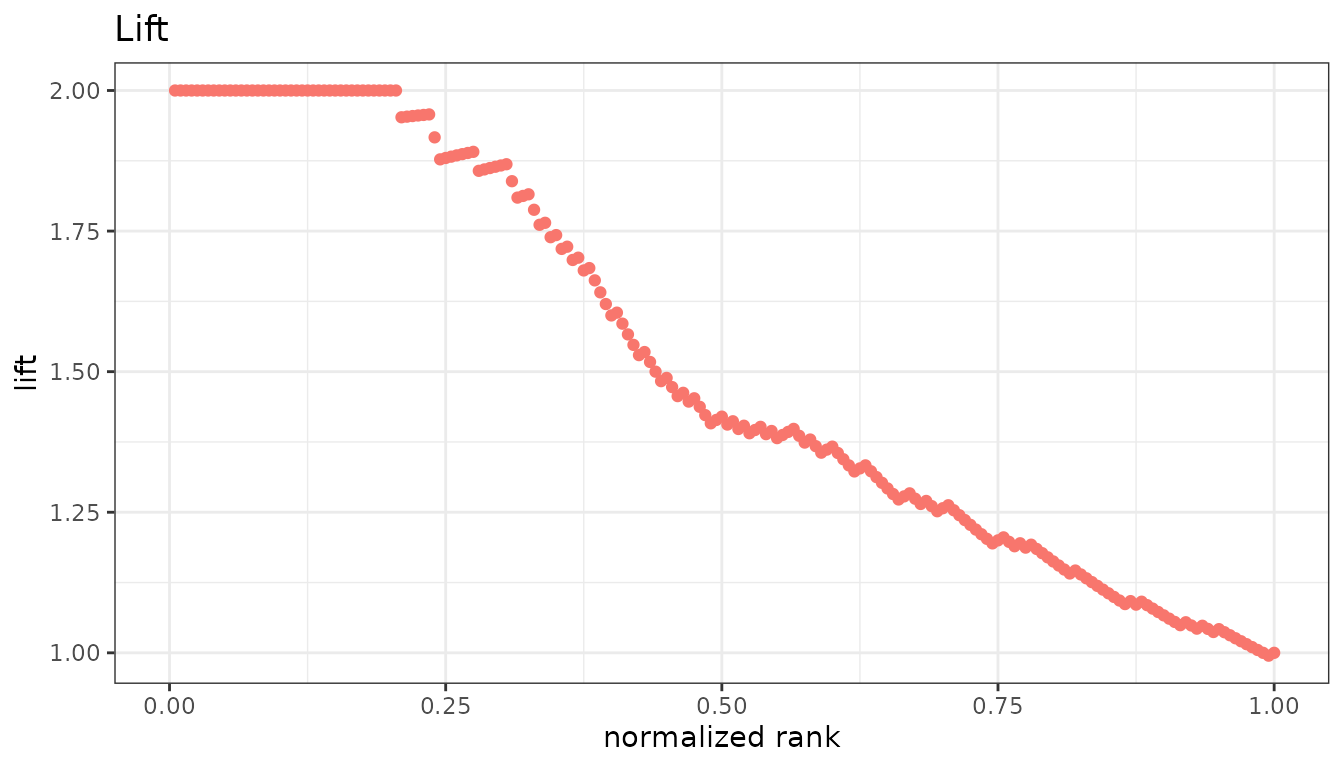
Likelihood ratios
| Measure | Formula | Range |
|---|---|---|
positive_likelihood_ratio |
sensitivity / FPR | 0 upward |
negative_likelihood_ratio |
FNR / specificity | 0 upward |
These are the two halves of the odds ratio above - LR+ divided by LR-
is exactly odds - and they are worth keeping apart because
they answer different questions. LR+ is how much a positive prediction
multiplies the odds that a case really is positive; LR- is how much a
negative prediction multiplies them. A test can be worth using on the
strength of one alone, a large LR+ to confirm or a small LR- to rule
out, and the odds ratio, being the quotient, hides which of the two is
doing the work.
Both are ratios of rates rather than of counts, so neither moves when the prevalence does. That is what lets a value measured on one population be carried to another, and it is also the catch: a cutoff with an excellent LR+ still flags mostly false positives if positives are rare enough. The measure that answers that question is precision, on the confusion-matrix page.
lrs <- evalmod(
  scores = samps$scores, labels = samps$labels,
  mode = "basic",
  metrics = c("positive_likelihood_ratio", "negative_likelihood_ratio")
)

autoplot(lrs, "positive_likelihood_ratio")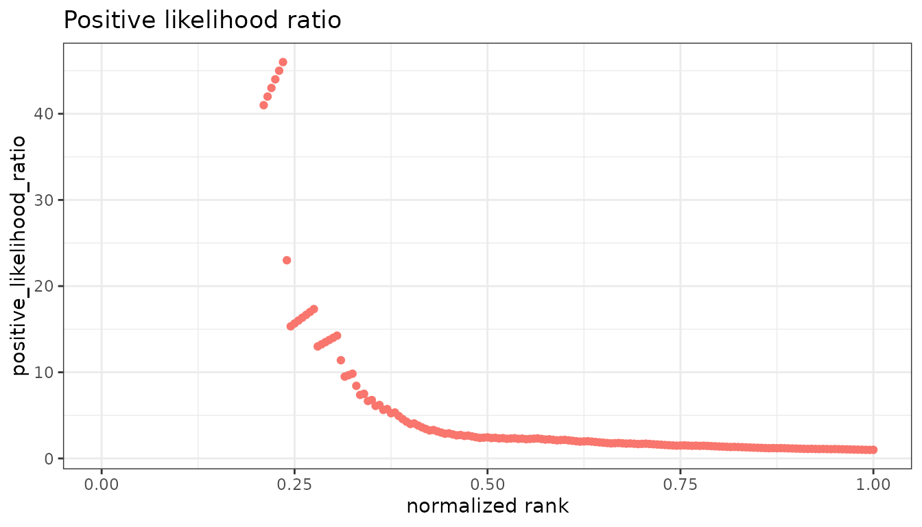
Cost
cost weights the two kinds of error separately:
(cost_fp x FP + cost_fn x FN) / all
With the default weights of 1 it is the error rate. Set the weights to what the two mistakes actually cost you, and the minimum of the curve is the cutoff to use.
costs <- evalmod(
  scores = samps$scores, labels = samps$labels,
  mode = "basic", metrics = "cost",
  cost_fp = 3, cost_fn = 0.5
)

autoplot(costs, "cost")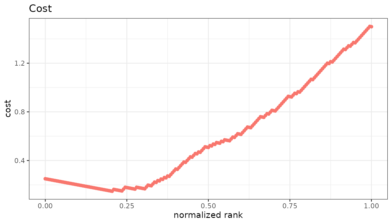
The measure is not normalized, following ROCR, so its
scale is the scale of the weights you gave.
Information
| Measure | What it is | Range |
|---|---|---|
mi |
Mutual information between prediction and truth, in bits | 0 to 1 |
chisq |
Pearson chi-square of the 2x2 table, n x mcc^2
|
0 upward |
Both ask how far the table is from independence rather than how good the predictions are. They are symmetric: a perfectly wrong classifier scores as high as a perfectly right one.
SAR
sar is the mean of three things - accuracy, the area
under the ROC curve, and one minus the root mean squared error -
proposed as a single summary that is harder to game than any one of
them.
The RMSE part reads the values of the scores rather than their ranks,
so sar needs scores that are probabilities between 0 and 1.
Given anything else it warns and returns NA, and every
other measure asked for in the same call is still returned.
Where values are undefined
Several of these are undefined at the very top and bottom of the ranking, where the 2x2 table has an empty cell.
-
oddsandchisqareNAthere. Some other tools report an infinity or aNaN;precrecreportsNA, as it already does for the undefined end of precision and NPV. - The likelihood ratios are
NAover a longer stretch than the others, and not only at the ends.positive_likelihood_ratiodivides by the false positive rate, which is 0 for every cutoff above the highest-scoring negative, andnegative_likelihood_ratiodivides by the specificity, which is 0 from the point where every negative has been flagged onward. -
miis0there rather thanNA. A cutoff that predicts one class for everything carries no information about the labels, so the value is defined and it is zero.